跟着Nature microbiology学作图：R语言ggplot2分组箱线图/wilcox秩和检验

论文

A high-quality genome compendium of the human gut microbiome of Inner Mongolians

2023Naturemicrobiology--Ahigh-qualitygenomecompendiumofthehumangutmicrobiomeofInnerMongolians4.pdf

论文中大部分作图数据都有，争取把论文中的图都复现一下

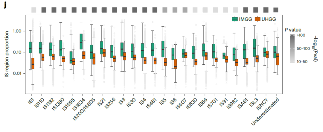
今天的推文我们试着复现一下论文中的Figure3j

部分示例数据截图

读取数据

library(readxl)
library(ggplot2)
library(tidyverse)



datj<-read_excel("data/20230305/41564_2022_1270_MOESM6_ESM.xlsx",
                 sheet = "Fig3j")
head(datj)
colnames(datj)

分组箱线图

p<-ggplot(data=datj,aes(x=`ID type`,
                     y=log10(`IS region proportion`)))+
  geom_boxplot(aes(fill=Database),
               outlier.shape = 1,
               outlier.colour = "gray",
               outlier.alpha = 0.2)+
  theme_bw()+
  theme(panel.grid = element_blank(),
        axis.text.x = element_text(angle=60,hjust=1,vjust=1),
        legend.position = "bottom")+
  scale_fill_manual(values = c("IMGG"="#1b9e77",
                               "UHGG"="#d95f02"),
                    name=NULL)+
  labs(x=NULL,y="IS region proportion")+
  scale_y_continuous(breaks = c(-2,-1,0),
                     labels = c("0.01","0.10","1.00"))
p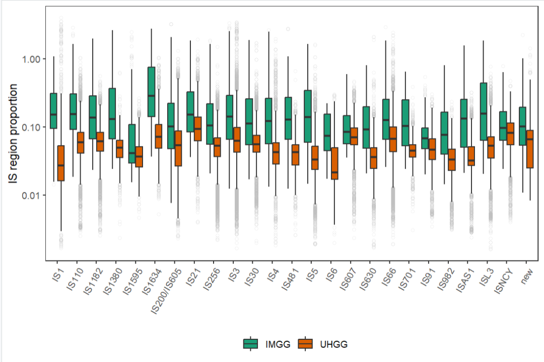

给箱线图添加上下小短线

ggplot_build(p)$data[[1]] %>% select(x,ymin,ymax) -> errorbar.df



p.bottom<-p+
  geom_segment(data = errorbar.df,
               aes(x=x-0.15,xend=x+0.15,y=ymin,yend=ymin))+
  geom_segment(data = errorbar.df,
               aes(x=x-0.15,xend=x+0.15,y=ymax,yend=ymax))

p.bottom

关于箱线图的图注英文

Statistical difference was tested by Wilcoxon rank-sum test (two-sided). For all boxplots, the boxes represent the interquartile range, the lines inside the boxes represent the medians, and the whiskers denote the lowest and highest values within 1.5 times the interquartile range.

分组做wilcox秩和检验

datj %>% 
  pull(`ID type`) %>% 
  unique() -> group.info

pvalue.df<-tibble(x=character(),
               pvalue=numeric())

for(info in group.info){
  datj %>% 
    filter(`ID type`==info) -> tmp.df
  wilcox.test(`IS region proportion`~`Database`,
              data=tmp.df) -> a
  add_row(pvalue.df,
          x=info,
          pvalue=a$p.value) -> pvalue.df
}

min_p<-min(pvalue.df %>% filter(pvalue !=0) %>% 
      pull(pvalue))
pvalue.df %>% 
  mutate(new_p=case_when(
    pvalue == 0 ~ min_p,
    TRUE ~ pvalue
  )) ->pvalue.df

画图展示结果

library(RColorBrewer)
scale_color_distiller()
p.top<-ggplot(data = pvalue.df,aes(x=x,y=1))+
  geom_point(size=5,shape=15,
             aes(color=-log10(new_p)))+
  scale_color_distiller(palette = "Greys",
                        direction = 1,
                        name="-log10(Pval)")+
  theme_void()+
  theme(legend.position = "top",
        legend.key.size = unit(5,'mm'),
        legend.text = element_text(size=10))+
  guides(color=guide_colorbar(title.position = "top",
                              title.hjust = 0.5,
                              barwidth = 20))

p.top

最后是拼图

library(patchwork)

p.top+
  p.bottom+
  plot_layout(ncol = 1,heights = c(1,5))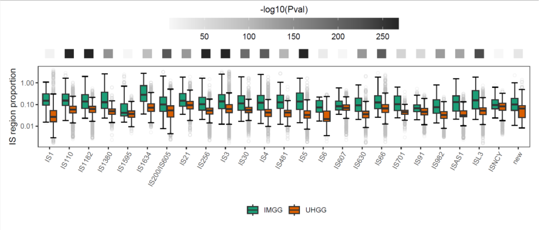

推文记录的是自己的学习笔记，很可能存在错误，请大家批判着看

示例数据和代码可以给推文打赏1元获取