
论文
The evolution of human altriciality and brain development in comparative context
数据代码
论文中的数据和代码都有,看论文,然后对应数据和代码,应该能更好的理解论文的内容。今天的推文我们复现一下论文中的Figure1bcef 云雨图
这里用到的是smplot2这个R包
对应的github主页是 https://github.com/smin95/smplot2
还有专门的文档介绍这个R包的用法 https://smin95.github.io/dataviz/
读取数据
library(tidyverse)
#devtools::install_github('smin95/smplot2')
library(smplot2)
mammals<-read.table("data/20231205/final_compilation with percentage values.R1.csv",
                    header=T,sep=",",row.names=1)

colnames(mammals)

mammals %>%
  select(NeoBody,AdultBody,BodyRatio) %>%
  head()

mammals %>% pull(Order2) %>% table()

mammals %>% pull(Over500gr) %>% table()

ordercolors<-c("coral1","lightslateblue","olivedrab3",
               "goldenrod1","lightgray")
mammals$Order2 <- factor(mammals$Order2,
                         levels = c("Artiodactyla", "Carnivora",
                                    "Primates", "Rodentia", "Others"))

mammals$Over500gr<-factor(mammals$Over500gr,
                          levels = c("Perissodactyls","Cetaceans",
                                     "Arctoids","Hominids","Elephants","Others"))
figure1b
ggplot(mammals, aes(x = Order2, y = 100*BodyRatio, fill = Order2)) +
  ylim(0,100)+
  labs(y="Body Proportion (%)",x="")+
  scale_fill_manual(values = ordercolors)+
  sm_raincloud() +
  theme(text = element_text(size = 13))+
  scale_x_discrete(labels = c('Artio','Carn','Prim','Rod','Others'))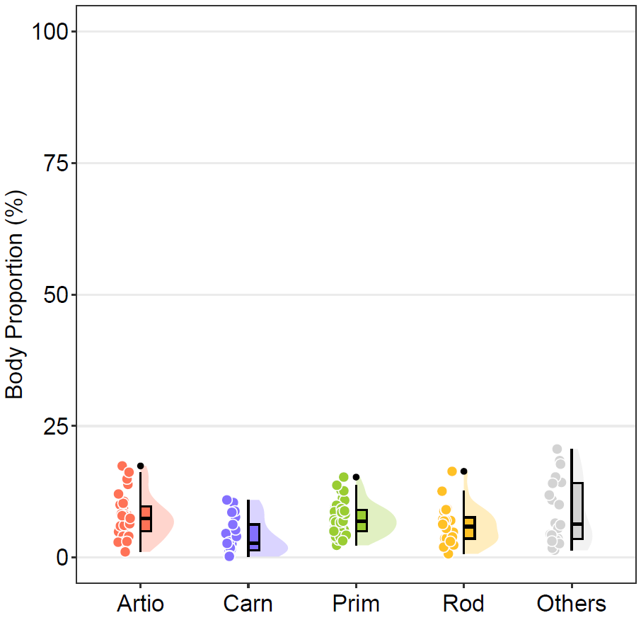

这个配色还挺好看的,另外3个图和这个图基本一致,这个R包还挺好用的,一行代码就出这个图
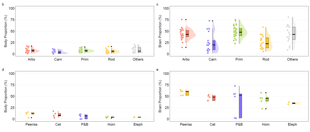
另外3个图的代码
ggplot(mammals, aes(x = Order2, y = 100*BrainRatio, fill = Order2)) +
  ylim(0,100)+
  labs(y="Brain Proportion (%)",x="")+
  scale_fill_manual(values = ordercolors)+
  sm_raincloud() +
  theme(text = element_text(size = 13))+
  scale_x_discrete(labels = c('Artio','Carn','Prim','Rod','Others'))


ggplot(mammals %>%
         filter(Over500gr != "Others"),
       aes(x = Over500gr, y = 100*BrainRatio, fill = Order2)) +
  ylim(0,100)+
  labs(y="Brain Proportion (%)",x="")+
  scale_fill_manual(values = ordercolors)+
  sm_raincloud() +
  theme(text = element_text(size = 13))+
  scale_x_discrete(labels = c('Peeriss','Cet','P&B','Hom','Eleph'))


ggplot(mammals %>%
         filter(Over500gr != "Others"),
       aes(x = Over500gr, y = 100*BodyRatio, fill = Order2)) +
  ylim(0,100)+
  labs(y="Body Proportion (%)",x="")+
  scale_fill_manual(values = ordercolors)+
  sm_raincloud() +
  theme(text = element_text(size = 13))+
  scale_x_discrete(labels = c('Peeriss','Cet','P&B','Hom','Eleph'))
四个图组合到一起
fig1b<-ggplot(mammals, aes(x = Order2, y = 100*BodyRatio, fill = Order2)) +
  ylim(0,100)+
  labs(y="Body Proportion (%)",x="")+
  scale_fill_manual(values = ordercolors)+
  sm_raincloud() +
  theme(text = element_text(size = 13))+
  scale_x_discrete(labels = c('Artio','Carn','Prim','Rod','Others'))

fig1c<-ggplot(mammals, aes(x = Order2, y = 100*BrainRatio, fill = Order2)) +
  ylim(0,100)+
  labs(y="Brain Proportion (%)",x="")+
  scale_fill_manual(values = ordercolors)+
  sm_raincloud() +
  theme(text = element_text(size = 13))+
  scale_x_discrete(labels = c('Artio','Carn','Prim','Rod','Others'))

fig1d<-ggplot(mammals %>%
         filter(Over500gr != "Others"),
       aes(x = Over500gr, y = 100*BodyRatio, fill = Order2)) +
  ylim(0,100)+
  labs(y="Body Proportion (%)",x="")+
  scale_fill_manual(values = ordercolors)+
  sm_raincloud() +
  theme(text = element_text(size = 13))+
  scale_x_discrete(labels = c('Peeriss','Cet','P&B','Hom','Eleph'))

fig1e<-ggplot(mammals %>%
         filter(Over500gr != "Others"),
       aes(x = Over500gr, y = 100*BrainRatio, fill = Order2)) +
  ylim(0,100)+
  labs(y="Brain Proportion (%)",x="")+
  scale_fill_manual(values = ordercolors)+
  sm_raincloud() +
  theme(text = element_text(size = 13))+
  scale_x_discrete(labels = c('Peeriss','Cet','P&B','Hom','Eleph'))

library(patchwork)

fig1b+fig1c+fig1d+fig1e+
  plot_annotation(tag_levels = list(c("b","c","d","e")))
示例数据和代码可以到论文中下载,或者给推文打赏一元获取我整理好的代码
声明:文中观点不代表本站立场。本文传送门:https://eyangzhen.com/386149.html